Merge Sort | Pseudo Code of Merge Sort | Merge Sort in Data Structure | Divide and Conquer Approach
The Merge Sort algorithm closely follows the Divide and Conquer paradigm (pattern) so before moving on merge sort let us see Divide and Conquer Approach.
“The Divide and Conquer Approach”
We have wide range of algorithm. For insertion sort, we used an incremental approach and one can use “Divide and Conquer” approach to design an algorithm to sort whose running time in worst case is much less than the worst case of insertion sort.
The Advantage of divide and conquer algorithm is that you can decide running time easily.
There are many algorithms which are recursive in structure to solve a given problem and they call themselves recursively one / more times to deal with related sub-problems. These type of algorithms typically follow a “Divide and Conquer” approach, first break the problem into several sub-problems recursively and then they combine these solutions to generate a solution of the original problem.
The divide and conquer approach involves three main steps :
- Divide : Here we Divides problem into a no. of sub-problems having smaller instances of the same problem.
- Conquer : Then we Conquer the sub-problems by solving them recursively.
- Combine : And in last, We Combines the solutions of the sub-problems into the solution for the original problem.
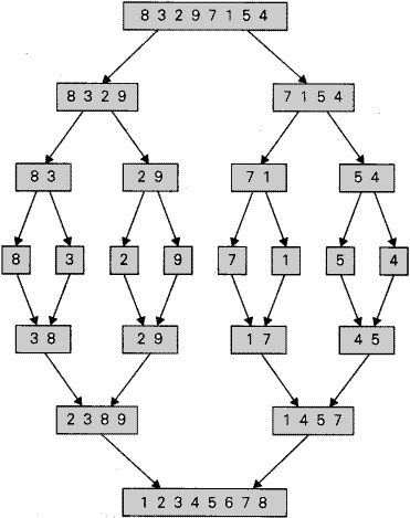
Let us see Divide and Conquer approach in Merge Sort “
- Divide : First divides the n element sequence into two sub sequences having size n / 2 elements each.
- Conquer : Then sort the each sub sequences recursively using merge sort.
- Combine : Then merge the two sub sequences which are sorted to produce the sorted answer.
Tracing of Merge Sort :
| //Algorithm of Merge Sort |
MERGE-SORT(A, p, r)
|
MERGE (A, p, q, r)
|

